The Histogramming Module
This module contains classes for histogramming.
We’ll cover the classes and their functionalities by directly using them in different examples.
The Histogram Classes
This package provides full support for N-Dimensional histograms: HistND.
But for your convenience, there are also classes derived from HistND
that are more convenient to use when you need lower dimensional histograms:
Regardles of the histogram’s dimension, the bins are all floats and equal width on the axis. As such, for the moment the histograms don’t support non-linear axis such as logarithmic axis.
Creating Histograms
To create a histogram we must say how the bins are distributed on each axis (per dimension). For each dimension of the histogram, the expected information is: the number of bins per axis, the minimum value on the axis of the lowest bin and the maximum value on the axis of the highest bin.
importing the library
But first we must import the histogram module:
from qksplot.hist import *
This command imports all classes defined in qksplot.hist module, more precisly the classes for 1D, 2D, 3D and ND histograms.
1D histogram
The easiest histograms to create are one dimensional (Hist1D):
h = Hist1D(100, -3.0, 3.0)
Above we created a 1D histogram that contains 100 bins starting from -3.0 to 3.0.
2D histogram
To create two dimensional histograms (Hist2D) it gets a bit complex, because we must explicitly say how the bins are distributed on 2 axis.:
h2 = Hist2D(100, -3, 3, 60, 0, 1000)
Here, we recongnize the first 3 arguments as representing the bin distribution on the first axis/dimension as we did previously for h . For the second axis, we can see that it has 60 bins starting from 0 and grow equally spaced till 1000.
3D histogram
A bit more complex is to create three dimensional histograms (Hist3D):
h3 = Hist3D(100, -3, 3, 60, 0, 1000, 80, -5, 3)
To construct 3D histograms is basically the same as for 2D histograms with the added difference we need 3 more arguments to specify bin distribution on the third axis. Pretty simple!
ND histogram
When we want to go to higher dimensions then 3 we must use the N-Dimensional histogram class (HistND). Here, the interface is a bit different since we must deal
with N values for each parameter from the bin distribution. For this reason we must use arrays or lists:
hN = HistND( N, minBins, maxBins, nBins)
Where N is the number of dimensions and the other arguments are arrays/lists. Where we understand that the ith element represents its value on ith dimension/axis. For example, a 5 dimensional histogram:
N=5
mins = [0,0,0,0,0]
maxis = [5,6,8,8,8]
nbins = [5,6,8,10,10]

h5 = HistND(N, mins, maxis, nbins)
or, simply:
h5 = HistND(5, [0,-1,0,2,1], [5,6,8,8,11], [5,6,8,10,10])
We interpret as:
- the histogram has 5 dimensions
- the first axis has 5 bins starting from 0 till 5
- the second axis has 6 bins starting from -1 till 6
- the third axis has 8 bins starting from 0 till 8
- the fourth axis has 10 bins starting from 2 till 8
- the fifth axis has 10 bins starting from 1 till 11
Warning
N-dimensional histogramming is very demanding of memory: a HistND with 8 dimensions and 100 bins per dimension needs more than 2.5GB of RAM!
the title of the histogram
There is one more argument that all histogram classes share it. We didn’t show it because its not important to the histogramming functionality, the argument is the title of the histogram. This argument is only used to keep it around untill the moment of drawing the histogram. That’s his only functionality.
Let’s see an example on how to use title it in the constructor:
h2 = Hist2D(100, -3, 3, 60, 0, 1000, title="Nch vs Pt")
Filling
A histogram is useless if it is not filled.
In this section we present the filling methods of histograms of different dimensions. First, we start with the simples methods. We kept the more advanced functionality in a subsection of it own at the end of this section.
1D histogram
One can fill a 1-dimensional histogram by simply calling the fill method:
h.fill(val)
This methods automatically searches the bin that can contain the value val and adds 1 to the counter of the bin.
You can specify a weight using the named argument weight:
h.fill(val, weight=w)
Which automatically searches the bin that can contain the value val and adds the weight w to the counter of the bin.
Note
Using the simple fill methods there is no need to say which bin you want filled, just a position that is inside a bin.
2D histogram
The 2D histograms are filled similarly to 1D case, with the exception this time we must take care of 2 axis:
h2.fill(valX, valY)
Now, the fill method automatically searches the bin on the first axis (alternatively called X-axis) that can contain the value valX and the bin on the second axis (aka called Y-axis) that can contain the value valY and adds 1 to the counter of the bin.
Note
You may wonder: since there are bins on X-axis and bins on Y-axis which bin its actually filled?
The answer: None of those. Because those bins don’t exists for the reason that internally, the histogram classes contain N-dimensional cells also known as global linear bins as you may find it in other parts of the documentation. These cells represent the intersection of the bins from all axis.
Respectively, you can specify a weight:
h2.fill(valX, valY, weight=w)
3D histogram
Its obvious by now, the fill method for the 3D histogram is:
h3.fill(valX, valY, valZ)
and with a weight:
h3.fill(valX, valY, valZ, weight=w)
ND histogram
An ND histogram a.k.a “N dimensional” histogram can be filled just like any other lower dimensional histogram: list “n” arguments to fill method, where n is the number of dimensions of the histogram
# fill a 5 dimensional histogram
h.fill(3.46, -0.33, 7.1, 2.28, 9)  # 5D means listing 5 arguments

# fill a 7 dimensional histogram
h.fill(3.46, -0.33, 7.1, 2.28, 9, 2.76, 3.1415)  # 7D means listing 7 arguments

# fill a 11 dimensional histogram
h.fill(3.46, -0.33, 7.1, 2.28, 9, 2.76, 3.1415, 6.67, 2.998, 0.0, 1.0)   # 11D means listing 1 arguments

# or, fill 5D hist with a weight
h.fill(3.46, -0.33, 7.1, 2.28, 9, weight=2.33)   # 5D means listing 5 arguments and weight as keyword argument
Since the fill method accepts arbitrary argument list, we can also use tuples or lists but care must be taken to first unpack them:
d = [3.46, -0.33, 7.1, 2.28, 9, 2.76, 3.1415, 6.67, 2.998, 0.0, 1.0] # d has 11 values since a 11D hist needs 11 values
h11.fill(*d) # use * to unpack a list or tuple
Other Filling Methods
There are more ways to fill histograms. The methods below are available to all histograms, regardless of its dimension.
Use fill_pos when you know the position on each axis:
p = [1,0,100,2,86,47]
hist.fill_pos(*p)

# with weight:
w = 34.2
hist.fill_pos(*p, weight=w)
Use fill_bins when you know the bins ids on each axis:
mbins = [1,0,100,2,86,47]
hist.fill_bins(*mbins)

# with weight:
w = 34.2
hist.fill_bins(*mbins, weight=w)
Note
The argument is a list of bin indexes. The dimension of the list must be the same as the dimension of the histogram. The bin indexes start from 0 to MaxBinIndex-1. MaxBinIndex is known when creating the histogram.
Use fill_cell when you know the cell index (global bin idex):
icell = 34
hist.fill_cell(icell)

# with a weight:
w = 2.2
hist.fill_cell(icell, weight=w)
Note
The cell index starts from 0 to MAX_CELL_IDX, where MAX_CELL_IDX is the product of all the bin counters from all dimensions. Meaning for a 5D histogram that contains nbins=[5,6,8,10,10] the MAX_CELL_IDX=5*6*8*10*10
Operations
The histograms in this package support multiple operations done on them, such as Scaling, Adding, Substracting, Multiplying and Dividing between histograms.
Scaling
Any histogram, whether its 1D, 2D, 3D or ND, can be scaled by a factor using the scale method.
Take the following example:
# create a 1D histogram
myhist = Hist1D(10, 0, 10)

# fill the histogram
for x in range(100):
        r = random.uniform(0,10)

        myhist.fill(r)

# scale the histogram's bins by 2.3
myhist.scale(2.3)
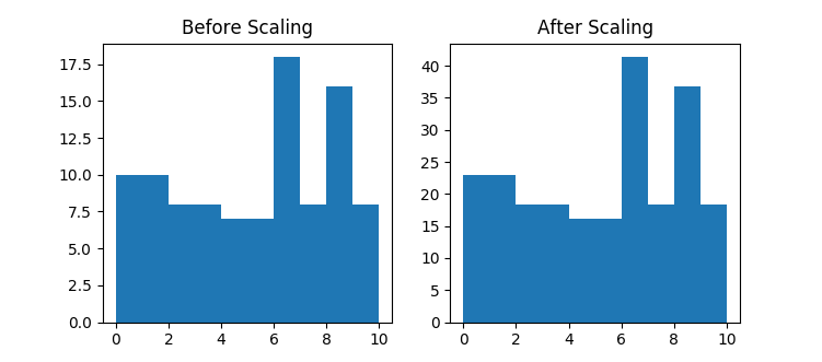
This method multiplies the internal bins (cells) by the value specified in the argument. The effect is visible in the above image where the vertical axis presents different values. Check a full example Scaling a histogram
Adding histograms
Histograms can be added by simply using the + operator:
# add 2 histograms
hSum = h1 + h2
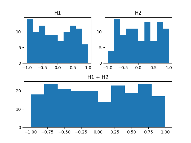
The plot of adding 2 histograms (top) and showing the resulted histogram (below). The plot was generated by the full example from How to Add two histograms
Substracting
Histograms can be substracted by simply using the - operator:
# substruct 2 histograms
hDiff = h1 - h2
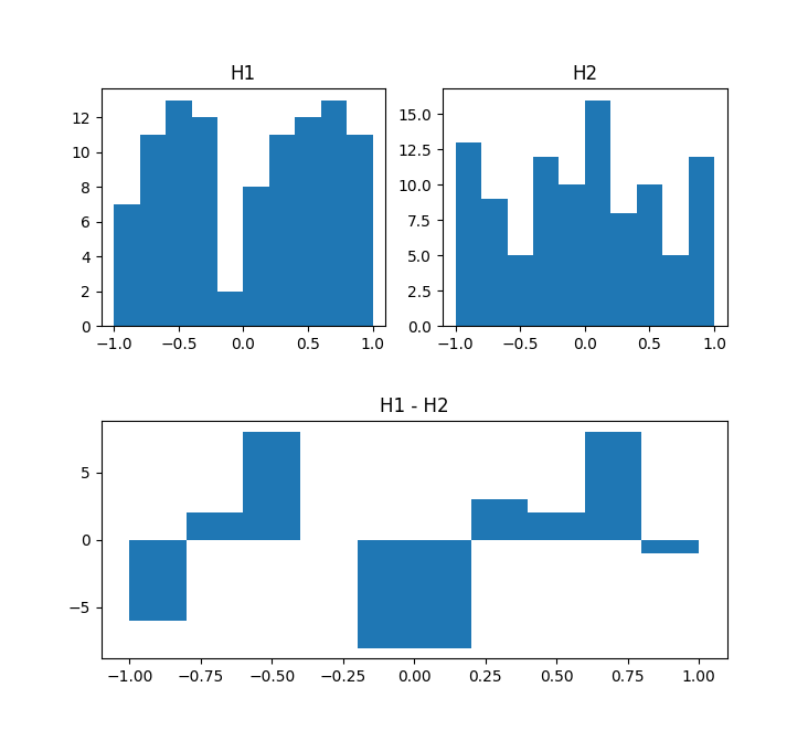
The plot of substracting a histogram from another (top) and showing the resulted histogram (below). The plot was generated by the full example from How to Substract histograms
Multiplying
Histograms can be multiplied by simply using the * operator:
# multiply 2 histograms
hDiff = h1 * h2
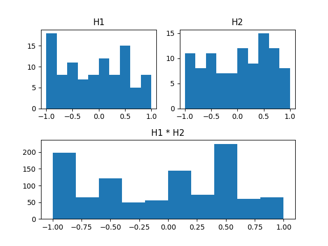
The plot of multiplying two histogram from another (top) and showing the resulted histogram (below). The plot was generated by the full example from How to Multiply histograms
Dividing
Histograms can be divided by simply using the / operator:
# divide 2 histograms
hDiff = h1 / h2
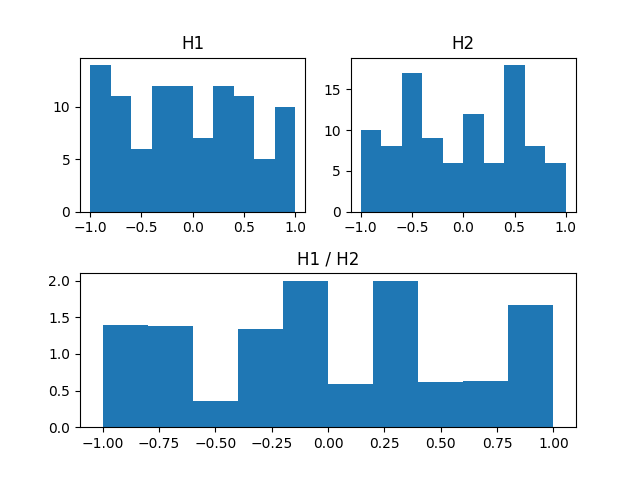
The plot of dividing two histogram from another (top) and showing the resulted histogram (below). The plot was generated by the full example from How to Divide histograms
Integrating
You can integrate the histogram (do the sum of the values of its internal cells multiplied with the volume described by its bins).
To do the integration you have 3 ways or methods, they differ by the meaning of their arguments.
Use integral_over_pos to do the integration over 2 position:
p = [0.33, 4.61, 78.29, 11.2]
q = [1.22, 3.2, 88, 27.0]
h.integral_over_pos(p, q)
here h can be any dimensional histogram. The arguments p and q are two positions (arrays) and p < q.
Use integral_over_bins when you know the bins:
b1 = [0, 4, 5]
b2 = [1, 1, 0]
h.integral_over_bins(b1, b2)
here h can be any dimensional histogram. The arguments b1 and b2 are bins positions (arrays) and b1 < b2.
Use integral when you know the two cell indexes:
c1 = 34
c2 = 90
h.integral(c1, c2)
here h can be any dimensional histogram. The arguments c1 and c2 are cell indexes (integers) and c1 < c2.
Projections
You can project any higher dimensional histogram to any lower dimensional histogram. The projection is also a histogram, containing less dimensions.
Projecting 2D histograms
Projecting 2D histograms is easy:
hproj = h2D.projection_x()
This projects a 2D histogram to its first axe (named x). The result hproj is a 1D histogram.
You can also project it on the second axe, called Y:
hproj = h2D.projection_y()
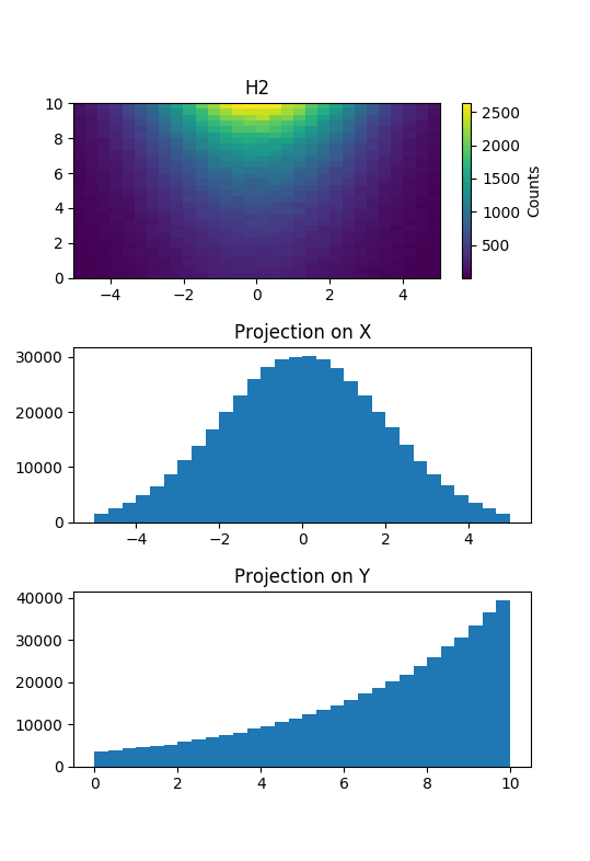
The 2D histogram above is projected along axes X and Y. See the full example How to Project histograms
Projecting 3D histograms
Besides the usual projecting methods as seen for 2D histograms (projection_x, projection_y) we get specific methods for 3D such as projection_z. Also, we can make projections on multiple planes defined by different combinations of axis.
Thus, we get a projection on XY plane:
hXYproj = h3D.projection_xy()
Or a projection on XZ plane:
hXZproj = h3D.projection_xz()
Or a projection on YZ plane:
hYZproj = h3D.projection_yz()
Projecting ND histograms
We’ve seen how easy is to do projections for lower dimensional histograms.
When projecting higher dimensional histograms (HistND) we must be more explicit and specify which dimensions we keep while projecting. For example, when we used projection_x to project a 2D or 3D histogram on the X axis, the projection operation does this: keep X axis and all the rest axis are projected. When we used projection_yz the projection operation keeps Y & Z axis and projects the rest (only X axis in this case).
We must recognize a general projection algorithm can not contain the letters for N-dimensional histograms, we do not have that many letters. For this reason, we must specify an variadic argument list as axis indexes the ones we want to keep. Axis indexis are just numbered as the first axis (called X) has index 0, Y is 1 and Z is 2, and so on.
Lets see some examples on how to project a 7 dimensional histogram:
# create a 7 dimensional histogram
h = HistND(7, [-1,0,0,0,0,0,0], [1,10,10,10,10,10,10], [10,10,10,10,10,10,10])

# code to fill the histogram
# ...
# ...
# ...

# create a projection on the first axis (aka X)
hXproj = h.projection(0)

# create a projection on the second axis (aka Y)
hYproj = h.projection(1)

# create a projection on the 7th axis
hproj = h.projection(6)

# create a projection on XY
hXYproj = h.projection(0,1)

# create a projection on X and the 5th axis
hX5proj = h.projection(0,4)

# create a projection on XYZ
hXYZproj = h.projection(0,1,2)

# create a projection on XYZ and the 5th & 7th axis
hproj = h.projection(0,1,2,4,6)
Drawing
The Histogramming module’s design is intended only for histogramming in order to let the user decide which library they prefer for plotting. Hence, this module has no drawing/plotting capabilities.
We recognized the need to plot easy and quickly and for this reason the qksplot package provides a separate module specifically created to quickly draw the histograms objects. Go read about it here.